
Video:
(Lightly edited) slides: https://intelligence.org/files/Factored-Set-Slides.pdf
(Part 1, Title Slides) · · · Finite Factored Sets
(Part 1, Motivation) · · · Some Context
 Scott: So I want to start with some context. For people who are not already familiar with my work:
- My main motivation is to reduce existential risk.
- I try to do this by trying to figure out how to align advanced artificial intelligence.
- I try to do this by trying to become less confused about intelligence and optimization and agency and various things in that cluster.
- My main strategy here is to develop a theory of agents that are embedded in the environment that they’re optimizing. I think there are a lot of open hard problems around doing this.
- This leads me to do a bunch of weird math and philosophy. This talk is going to be an example of some weird math and philosophy.
For people who are already familiar with my work, I just want to say that according to my personal aesthetics, the subject of this talk is about as exciting as Logical Induction, which is to say I’m really excited about it. And I’m really excited about this audience; I’m excited to give this talk right now.
(Part 1, Table of Contents) · · · Factoring the Talk
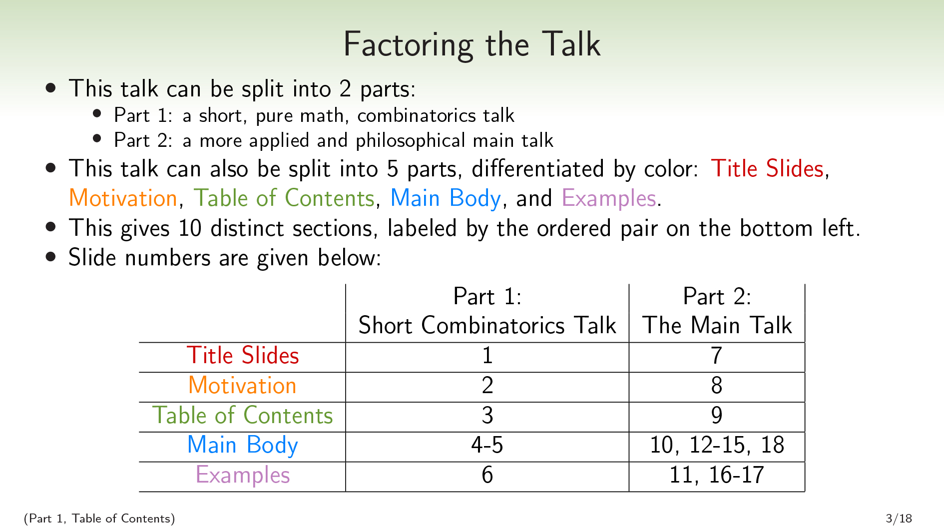 This talk can be split into 2 parts:
Part 1, a short pure-math combinatorics talk.
Part 2, a more applied and philosophical main talk.
This talk can also be split into 5 parts differentiated by color: Title Slides, Motivation, Table of Contents, Main Body, and Examples. Combining these gives us 10 parts (some of which are not contiguous):
| Part 1: Short Talk | Part 2: The Main Talk | |
| Title Slides | Finite Factored Sets | The Main Talk (It’s About Time) |
| Motivation | Some Context | The Pearlian Paradigm |
| Table of Contents | Factoring the Talk | We Can Do Better |
| Main Body | Set Partitions, etc. | Time and Orthogonality, etc. |
| Examples | Enumerating Factorizations | Game of Life, etc. |
(Part 1, Main Body) · · · Set Partitions
 All right. Here’s some background math:
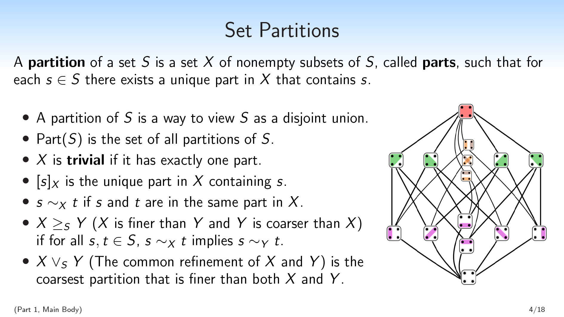
- A partition of a set \(S\) is a set \(X\) of non-empty subsets of \(S\), called parts, such that for each \(s∈S\) there exists a unique part in \(X\) that contains \(s\).
- Basically, a partition of \(S\) is a way to view \(S\) as a disjoint union. We have parts that are disjoint from each other, and they union together to form \(S\).
- We’ll write \(\mathrm{Part}(S)\) for the set of all partitions of \(S\).
- We’ll say that a partition \(X\) is trivial if it has exactly one part.
- We’ll use bracket notation, \([s]_{X}\), to denote the unique part in \(X\) containing \(s\). So this is like the equivalence class of a given element.
- And we’ll use the notation \(s∼_{X}t\) to say that two elements \(s\) and \(t\) are in the same part in \(X\).
You can also think of partitions as being like variables on your set \(S\). Viewed in that way, the values of a partition \(X\) correspond to which part an element is in.
Or you can think of \(X\) as a question that you could ask about a generic element of \(S\). If I have an element of \(S\) and it’s hidden from you and you want to ask a question about it, each possible question corresponds to a partition that splits up \(S\) according to the different possible answers.
We’re also going to use the lattice structure of partitions:
- We’ll say that \(X \geq_S Y\) (\(X\) is finer than \(Y\), and \(Y\) is coarser than \(X\)) if \(X\) makes all of the distinctions that \(Y\) makes (and possibly some more distinctions), i.e., if for all \(s,t \in S\), \(s \sim_X t\) implies \(s \sim_Y t\). You can break your set \(S\) into parts, \(Y\), and then break it into smaller parts, \(X\).
- \(X\vee_S Y\) (the common refinement of \(X\) and \(Y\) ) is the coarsest partition that is finer than both \(X\) and \(Y\) . This is the unique partition that makes all of the distinctions that either \(X\) or \(Y\) makes, and no other distinctions. This is well-defined, which I’m not going to show here.
Hopefully this is mostly background. Now I want to show something new.
(Part 1, Main Body) · · · Set Factorizations
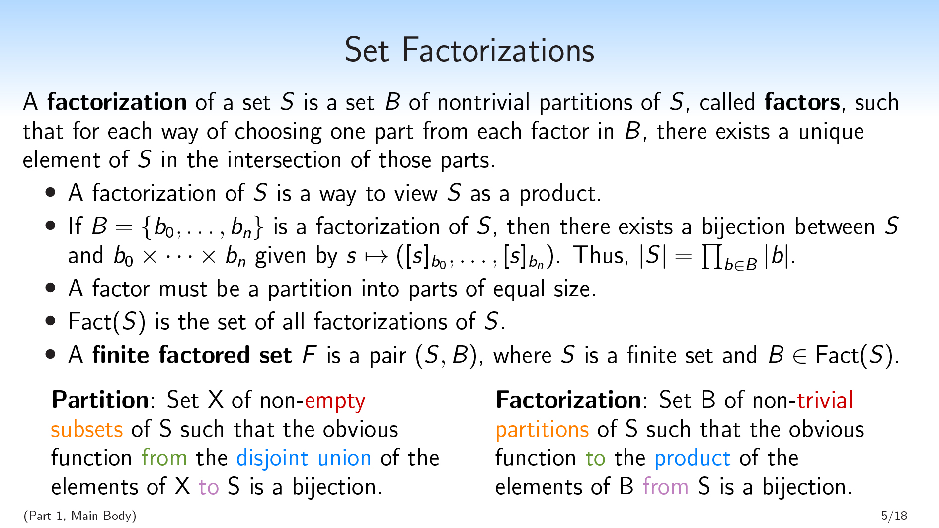 A factorization of a set \(S\) is a set \(B\) of nontrivial partitions of \(S\), called factors, such that for each way of choosing one part from each factor in \(B\), there exists a unique element of \(S\) in the intersection of those parts.
So this is maybe a little bit dense. My short tagline of this is: “A factorization of \(S\) is a way to view \(S\) as a product, in the exact same way that a partition was a way to view \(S\) as a disjoint union.”
If you take one definition away from this first talk, it should be the definition of factorization. I’ll try to explain it from a bunch of different angles to help communicate the concept.
If \(B=\{b_0,\dots,b_{n}\}\) is a factorization of \(S\) , then there exists a bijection between \(S\) and \(b_0\times\dots\times b_{n}\) given by \(s\mapsto([s]_{b_0},\dots,[s]_{b_{n}})\). This bijection comes from sending an element of \(S\) to the tuple consisting only of parts containing that element. And as a consequence of this bijection, \(|S|=\prod_{b\in B} |b|\).
So we’re really viewing \(S\) as a product of these individual factors, with no additional structure.
Although we won’t prove this here, something else you can verify about factorizations is that all of the parts in a factor have to be of the same size.
We’ll write \(\mathrm{Fact}(S)\) for the set of all factorizations of \(S\), and we’ll say that a finite factored set is a pair \((S,B)\), where \(S\) is a finite set and \(B \in \mathrm{Fact}(S)\).
Note that the relationship between \(S\) and \(B\) is somewhat loopy. If I want to define a factored set, there are two strategies I could use. I could first introduce the \(S\), and break it into factors. Alternatively, I could first introduce the \(B\). Any time I have a finite collection of finite sets \(B\), I can take their product and thereby produce an \(S\), modulo the degenerate case where some of the sets are empty. So \(S\) can just be the product of a finite collection of arbitrary finite sets.
To my eye, this notion of factorization is extremely natural. It’s basically the multiplicative analog of a set partition. And I really want to push that point, so here’s another attempt to push that point:
| A partition is a set \(X\) of non-empty subsets of \(S\) such that the obvious function from the disjoint union of the elements of \(X\) to \(S\) is a bijection. |
A factorization is a set \(B\) of non-trivial partitions of \(S\) such that the obvious function to the product of the elements of \(B\) from \(S\) is a bijection. |
I can take a slightly modified version of the partition definition from before and dualize a whole bunch of the words, and get out the set factorization definition.
Hopefully you’re now kind of convinced that this is an extremely natural notion.
| Andrew Critch: Scott, in one sense, you’re treating “subset” as dual to partition, which I think is valid. And then in another sense, you’re treating “factorization” as dual to partition. Those are both valid, but maybe it’s worth talking about the two kinds of duality.
Scott: Yeah. I think what’s going on there is that there are two ways to view a partition. You can view a partition as “that which is dual to a subset,” and you can also view a partition as something that is built up out of subsets. These two different views do different things when you dualize. Ramana Kumar: I was just going to check: You said you can start with an arbitrary \(B\) and then build the \(S\) from it. It can be literally any set, and then there’s always an \(S\)… Scott: If none of them are empty, yes, you could just take a collection of sets that are kind of arbitrary elements. And you can take their product, and you can identify with each of the elements of a set the subset of the product that projects on to that element. Ramana Kumar: Ah. So the \(S\) in that case will just be tuples. Scott: That’s right. Brendan Fong: Scott, given a set, I find it very easy to come up with partitions. But I find it less easy to come up with factorizations. Do you have any tricks for…? Scott: For that, I should probably just go on to the examples. Joseph Hirsh: Can I ask one more thing before you do that? You allow factors to have one element in them? Scott: I said “nontrivial,” which means it does not have one element. Joseph Hirsh: “Nontrivial” means “not have one element, and not have no elements”? Scott: No, the empty set has a partition (with no parts), and I will call that nontrivial. But the empty set thing is not that critical. |
I’m now going to move on to some examples.
(Part 1, Examples) · · · Enumerating Factorizations
Exercise! What are the factorizations of the set \(\{0,1,2,3\}\) ?
Spoiler space:
.
.
.
.
.
.
.
.
.
.
.
.
.
.
 First, we’re going to have a kind of trivial factorization:
\(\begin{split} \{ \ \ \{ \{0\},\{1\},\{2\},\{3\} \} \ \ \} \end{split} \begin{split} \ \ \ \ \underline{\ 0 \ \ \ 1 \ \ \ 2 \ \ \ 3 \ } \end{split}\)
We only have one factor, and that factor is the discrete partition. You can do this for any set, as long as your set has at least two elements.
Recall that in the definition of factorization, we wanted that for each way of choosing one part from each factor, we had a unique element in the intersection of those parts. Since we only have one factor here, satisfying the definition just requires that for each way of choosing one part from the discrete partition, there exists a unique element that is in that part.
And then we want some less trivial factorizations. In order to have a factorization, we’re going to need some partitions. And the product of the cardinalities of our partitions are going to have to equal the cardinality of our set \(S\) , which is 4.
The only way to express 4 as a nontrivial product is to express it as \(2 \times 2\) . Thus we’re looking for factorizations that have 2 factors, where each factor has 2 parts.
We noted earlier that all of the parts in a factor have to be of the same size. So we’re looking for 2 partitions that each break our 4-element set into 2 sets of size 2.
So if I’m going to have a factorization of \(\{0,1,2,3\}\) that isn’t this trivial one, I’m going to have to pick 2 partitions of my 4-element set that each break the set into 2 parts of size 2. And there are 3 partitions of a 4-element sets that break it up into 2 parts of size 2. For each way of choosing a pair of these 3 partitions, I’m going to get a factorization.
\(\begin{split} \begin{Bmatrix} \ \ \ \{\{0,1\}, \{2,3\}\}, \ \\ \{\{0,2\}, \{1,3\}\} \end{Bmatrix} \end{split} \begin{split} \ \ \ \ \ \ \ \ \ \ \ \ \ \ \ \ \begin{array} { |c|c|c|c| } \hline 0 & 1 \\ \hline 2 & 3 \\ \hline \end{array} \end{split}\)
\(\begin{split} \begin{Bmatrix} \ \ \ \{\{0,1\}, \{2,3\}\}, \ \\ \{\{0,3\}, \{1,2\}\} \end{Bmatrix} \end{split} \begin{split} \ \ \ \ \ \ \ \ \ \ \ \ \ \ \ \ \begin{array} { |c|c|c|c| } \hline 0 & 1 \\ \hline 3 & 2 \\ \hline \end{array} \end{split}\)
\(\begin{split} \begin{Bmatrix} \ \ \ \{\{0,2\}, \{1,3\}\}, \ \\ \{\{0,3\}, \{1,2\}\} \end{Bmatrix} \end{split} \begin{split} \ \ \ \ \ \ \ \ \ \ \ \ \ \ \ \ \begin{array} { |c|c|c|c| } \hline 0 & 2 \\ \hline 3 & 1 \\ \hline \end{array} \end{split}\)
So there will be 4 factorizations of a 4-element set.
In general you can ask, “How many factorizations are there of a finite set of size \(n\) ?”. Here’s a little chart showing the answer for \(n \leq 25\):
| \(|S|\) | \(|\mathrm{Fact}(S)|\) |
| 0 | 1 |
| 1 | 1 |
| 2 | 1 |
| 3 | 1 |
| 4 | 4 |
| 5 | 1 |
| 6 | 61 |
| 7 | 1 |
| 8 | 1681 |
| 9 | 5041 |
| 10 | 15121 |
| 11 | 1 |
| 12 | 13638241 |
| 13 | 1 |
| 14 | 8648641 |
| 15 | 1816214401 |
| 16 | 181880899201 |
| 17 | 1 |
| 18 | 45951781075201 |
| 19 | 1 |
| 20 | 3379365788198401 |
| 21 | 1689515283456001 |
| 22 | 14079294028801 |
| 23 | 1 |
| 24 | 4454857103544668620801 |
| 25 | 538583682060103680001 |
You’ll notice that if \(n\) is prime, there will be a single factorization, which hopefully makes sense. This is the factorization that only has one factor.
A very surprising fact to me is that this sequence did not show up on OEIS, which is this database that combinatorialists use to check whether or not their sequence has been studied before, and to see connections to other sequences.
To me, this just feels like the multiplicative version of the Bell numbers. The Bell numbers count how many partitions there are of a set of size \(n\). It’s sequence number 110 on OEIS out of over 300,000; and this sequence just doesn’t show up at all, even when I tweak it and delete the degenerate cases and so on.
I am very confused by this fact. To me, factorizations seem like an extremely natural concept, and it seems to me like it hasn’t really been studied before.
This is the end of my short combinatorics talk.
| Ramana Kumar: If you’re willing to do it, I’d appreciate just stepping through one of the examples of the factorizations and the definition, because this is pretty new to me.
Scott: Yeah. Let’s go through the first nontrivial factorization of \(\{0,1,2,3\}\): \(\begin{split} \begin{Bmatrix} \ \ \ \{\{0,1\}, \{2,3\}\}, \ \\ \{\{0,2\}, \{1,3\}\} \end{Bmatrix} \end{split} \begin{split} \ \ \ \ \ \ \ \ \ \ \ \ \ \ \ \ \begin{array} { |c|c|c|c| } \hline 0 & 1 \\ \hline 2 & 3 \\ \hline \end{array} \end{split}\) In the definition, I said a factorization should be a set of partitions such that for each way of choosing one part from each of the partitions, there will be a unique element in the intersection of those parts. Here, I have a partition that’s separating the small numbers from the large numbers: \(\{\{0,1\}, \{2,3\}\}\). And I also have a partition that’s separating the even numbers from the odd numbers: \(\{\{0,2\}, \{1,3\}\}\). And the point is that for each way of choosing either “small” or “large” and also choosing “even” or “odd”, there will be a unique element of \(S\) that is the conjunction of these two choices. In the other two nontrivial factorizations, I replace either “small and large” or “even and odd” with an “inner and outer” distinction. David Spivak: For partitions and for many things, if I know the partitions of a set \(A\) and the partitions of a set \(B\) , then I know some partitions of \(A+B\) (the disjoint union) or I know some partitions of \(A \times B\) . Do you know any facts like that for factorizations? Scott: Yeah. If I have two factored sets, I can get a factored set over their product, which sort of disjoint-unions the two collections of factors. For the additive thing, you’re not going to get anything like that because prime sets don’t have any nontrivial factorizations. |
All right. I think I’m going to move on to the main talk.
(Part 2, Title Slides) · · · The Main Talk (It’s About Time)
(Part 2, Motivation) · · · The Pearlian Paradigm
 We can’t talk about time without talking about Pearlian causal inference. I want to start by saying that I think the Pearlian paradigm is great. This buys me some crackpot points, but I’ll say it’s the best thing to happen to our understanding of time since Einstein.
I’m not going to go into all the details of Pearl’s paradigm here. My talk will not be technically dependent on it; it’s here for motivation.
Given a collection of variables and a joint probability distribution over those variables, Pearl can infer causal/temporal relationships between the variables. (In this talk I’m going to use “causal” and “temporal” interchangeably, though there may be more interesting things to say here philosophically.)
Pearl can infer temporal data from statistical data, which is going against the adage that “correlation does not imply causation.” It’s like Pearl is taking the combinatorial structure of your correlation and using that to infer causation, which I think is just really great.
| Ramana Kumar: I may be wrong, but I think this is false. Or I think that that’s not all Pearl needs—just the joint distribution over the variables. Doesn’t he also make use of intervention distributions?
Scott: In the theory that is described in chapter two of the book Causality, he’s not really using other stuff. Pearl builds up this bigger theory elsewhere. But you have some strong ability, maybe assuming simplicity or whatever (but not assuming you have access to extra information), to take a collection of variables and a joint distribution over those variables, and infer causation from correlation. Andrew Critch: Ramana, it depends a lot on the structure of the underlying causal graph. For some causal graphs, you can actually recover them uniquely with no interventions. And only assumptions with zero-measure exceptions are needed, which is really strong. Ramana Kumar: Right, but then the information you’re using is the graph. Andrew Critch: No, you’re not. Just the joint distribution. Ramana Kumar: Oh, okay. Sorry, go ahead. Andrew Critch: There exist causal graphs with the property that if nature is generated by that graph and you don’t know it, and then you look at the joint distribution, you will infer with probability 1 that nature was generated by that graph, without having done any interventions. Ramana Kumar: Got it. That makes sense. Thanks. Scott: Cool. |
I am going to (a little bit) go against this, though. I’m going to claim that Pearl is kind of cheating when making this inference. The thing I want to point out is that in the sentence “Given a collection of variables and a joint probability distribution over those variables, Pearl can infer causal/temporal relationships between the variables.”, the words “Given a collection of variables” are actually hiding a lot of the work.
The emphasis is usually put on the joint probability distribution, but Pearl is not inferring temporal data from statistical data alone. He is inferring temporal data from statistical data and factorization data: how the world is broken up into these variables.
I claim that this issue is also entangled with a failure to adequately handle abstraction and determinism. To point at that a little bit, one could do something like say:
“Well, what if I take the variables that I’m given in a Pearlian problem and I just forget that structure? I can just take the product of all of these variables that I’m given, and consider the space of all partitions on that product of variables that I’m given; and each one of those partitions will be its own variable. And then I can try to do Pearlian causal inference on this big set of all the variables that I get by forgetting the structure of variables that were given to me.”
And the problem is that when you do that, you have a bunch of things that are deterministic functions of each other, and you can’t actually infer stuff using the Pearlian paradigm.
So in my view, this cheating is very entangled with the fact that Pearl’s paradigm isn’t great for handling abstraction and determinism.
(Part 2, Table of Contents) · · · We Can Do Better
 The main thing we’ll do in this talk is we’re going to introduce an alternative to Pearl that does not rely on factorization data, and that therefore works better with abstraction and determinism.
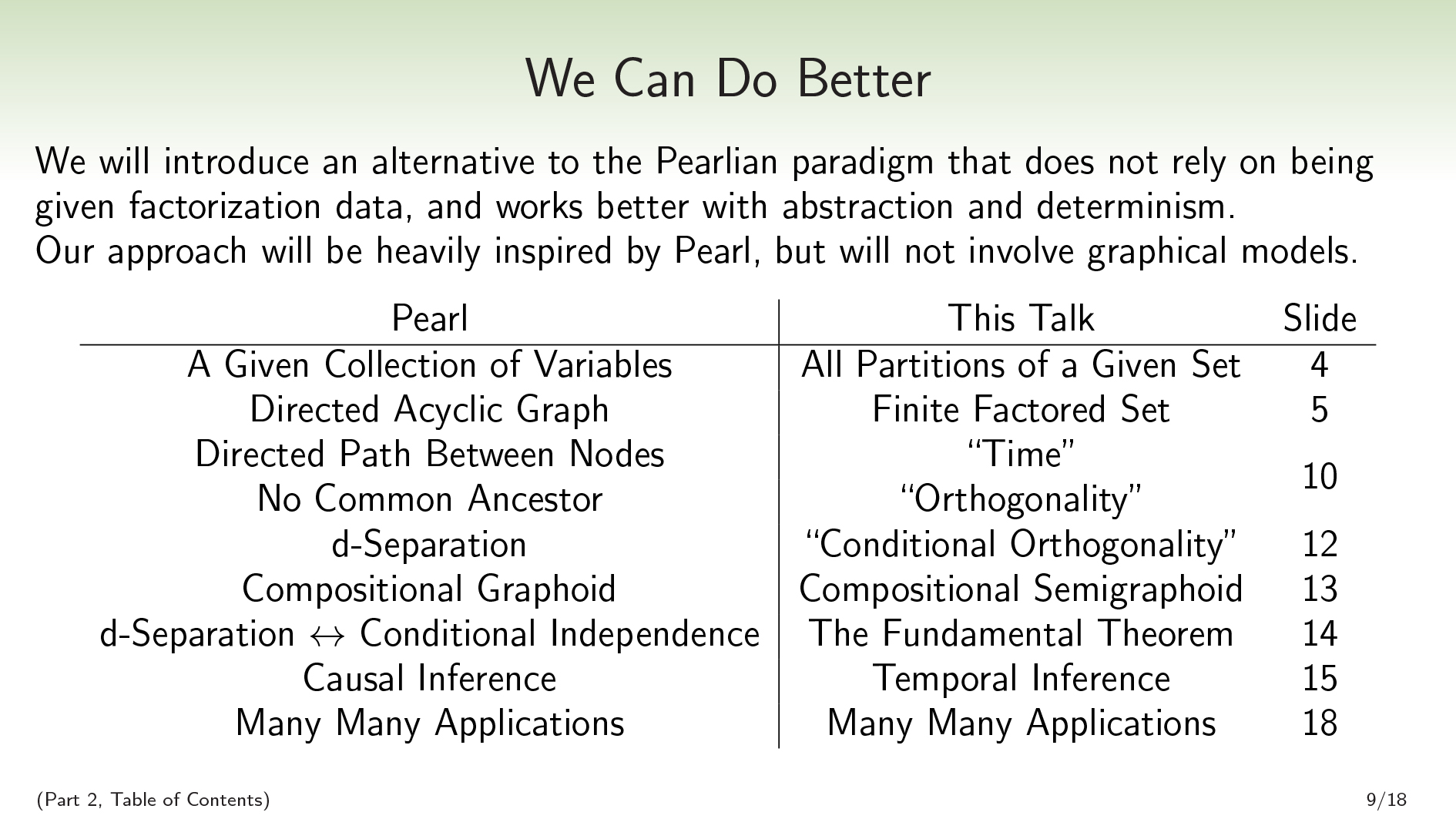
Where Pearl was given a collection of variables, we are going to just consider all partitions of a given set. Where Pearl infers a directed acyclic graph, we’re going to infer a finite factored set.
In the Pearlian world, we can look at the graph and read off properties of time and orthogonality/independence. A directed path between nodes corresponds to one node being before the other, and two nodes are independent if they have no common ancestor. Similarly, in our world, we will be able to read time and orthogonality off of a finite factored set.
(Orthogonality and independence are pretty similar. I’ll use the word “orthogonality” when I’m talking about a combinatorial notion, and I’ll use “independence” when I’m talking about a probabilistic notion.)
In the Pearlian world, d-separation, which you can read off of the graph, corresponds to conditional independence in all probability distributions that you can put on the graph. We’re going to have a fundamental theorem that will say basically the same thing: conditional orthogonality corresponds to conditional independence in all probability distributions that we can put on our factored set.
In the Pearlian world, d-separation will satisfy the compositional graphoid axioms. In our world, we’re just going to satisfy the compositional semigraphoid axioms. The fifth graphoid axiom is one that I claim you shouldn’t have even wanted in the first place.
Pearl does causal inference. We’re going to talk about how to do temporal inference using this new paradigm, and infer some very basic temporal facts that Pearl’s approach can’t. (Note that Pearl can also sometimes infer temporal relations that we can’t—but only, from our point of view, because Pearl is making additional factorization assumptions.)
And then we’ll talk about a bunch of applications.
| Pearl | This Talk |
| A Given Collection of Variables | All Partitions of a Given Set |
| Directed Acyclic Graph | Finite Factored Set |
| Directed Path Between Nodes | “Time” |
| No Common Ancestor | “Orthogonality” |
| d-Separation | “Conditional Orthogonality” |
| Compositional Graphoid | Compositional Semigraphoid |
| d-Separation ↔ Conditional Independence | The Fundamental Theorem |
| Causal Inference | Temporal Inference |
| Many Many Applications | Many Many Applications |
Excluding the motivation, table of contents, and example sections, this table also serves as an outline of the two talks. We’ve already talked about set partitions and finite factored sets, so now we’re going to talk about time and orthogonality.
(Part 2, Main Body) · · · Time and Orthogonality
 I think that if you capture one definition from this second part of the talk, it should be this one. Given a finite factored set as context, we’re going to define the history of a partition.
Let \(F = (S,B)\) be a finite factored set. And let \(X, Y \in \mathrm{Part}(S)\) be partitions of \(S\).
The history of \(X\) , written \(h^F(X)\), is the smallest set of factors \(H \subseteq B\) such that for all \(s, t \in S\), if \(s \sim_b t\) for all \(b \in H\), then \(s \sim_X t\).
The history of \(X\) , then, is the smallest set of factors \(H\) —so, the smallest subset of \(B\) —such that if I take an element of \(S\) and I hide it from you, and you want to know which part in \(X\) it is in, it suffices for me to tell you which part it is in within each of the factors in \(H\) .
So the history \(H\) is a set of factors of \(S\) , and knowing the values of all the factors in \(H\) is sufficient to know the value of \(X\) , or to know which part in \(X\) a given element is going to be in. I’ll give an example soon that will maybe make this a little more clear.
We’re then going to define time from history. We’ll say that \(X\) is weakly before \(Y\), written \(X\leq^F Y\), if \(h^F(X)\subseteq h^F(Y)\) . And we’ll say that \(X\) is strictly before \(Y\), written \(X<^F Y\), if \(h^F(X)\subset h^F(Y)\).
One analogy one could draw is that these histories are like the past light cones of a point in spacetime. When one point is before another point, then the backwards light cone of the earlier point is going to be a subset of the backwards light cone of the later point. This helps show why “before” can be like a subset relation.
We’re also going to define orthogonality from history. We’ll say that two partitions \(X\) and \(Y\) are orthogonal, written \(X\perp^FY\) , if their histories are disjoint: \(h^F(X)\cap h^F(Y)=\{\}\).
Now I’m going to go through an example.
(Part 2, Examples) · · · Game of Life
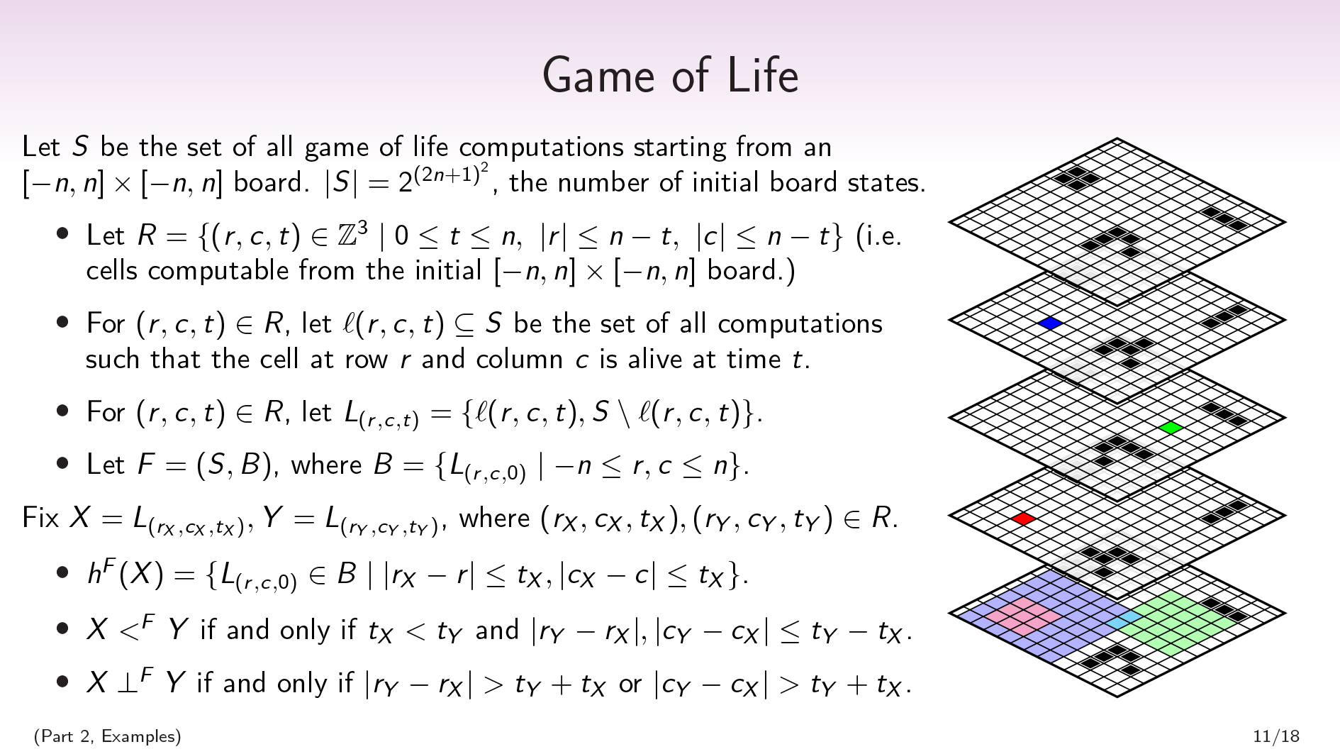 Let \(S\) be the set of all Game of Life computations starting from an \([-n,n]\times[-n,n]\) board.
Let \(R=\{(r,c,t)\in\mathbb{Z}^3\mid0\leq t\leq n,\ \) \(|r|\leq n-t,\ |c|\leq n-t\}\) (i.e., cells computable from the initial \([-n,n]\times[-n,n]\) board). For \((r,c,t)\in R\), let \(\ell(r,c,t)\subseteq S\) be the set of all computations such that the cell at row \(r\) and column \(c\) is alive at time \(t\).
(Minor footnote: I’ve done some small tricks here in order to deal with the fact that the Game of Life is normally played on an infinite board. We want to deal with the finite case, and we don’t want to worry about boundary conditions, so we’re only going to look at the cells that are uniquely determined by the initial board. This means that the board will shrink over time, but this won’t matter for our example.)
\(S\) is the set of all Game of Life computations, but since the Game of Life is deterministic, the set of all computations is in bijective correspondence with the set of all initial conditions. So \(|S|=2^{(2n+1)^{2}}\) , the number of initial board states.
This also gives us a nice factorization on the set of all Game of Life computations. For each cell, there’s a partition that separates out the Game of Life computations in which that cell is alive at time 0 from the ones where it’s dead at time 0. Our factorization, then, will be a set of \((2n+1)^{2}\) binary factors, one for each question of “Was this cell alive or dead at time 0?”.
Formally: For \((r,c,t)\in R\), let \(L_{(r,c,t)}=\{\ell(r,c,t),S\setminus \ell(r,c,t)\}\). Let \(F=(S,B)\), where \(B=\{L_{(r,c,0)}\mid -n\leq r,c\leq n\}\).
There will also be other partitions on this set of all Game of Life computations that we can talk about. For example, you can take a cell and a time \(t\) and say, “Is this cell alive at time \(t\)?”, and there will be a partition that separates out the computations where that cell is alive at time \(t\) from the computations where it’s dead at time \(t\).
Here’s an example of that:
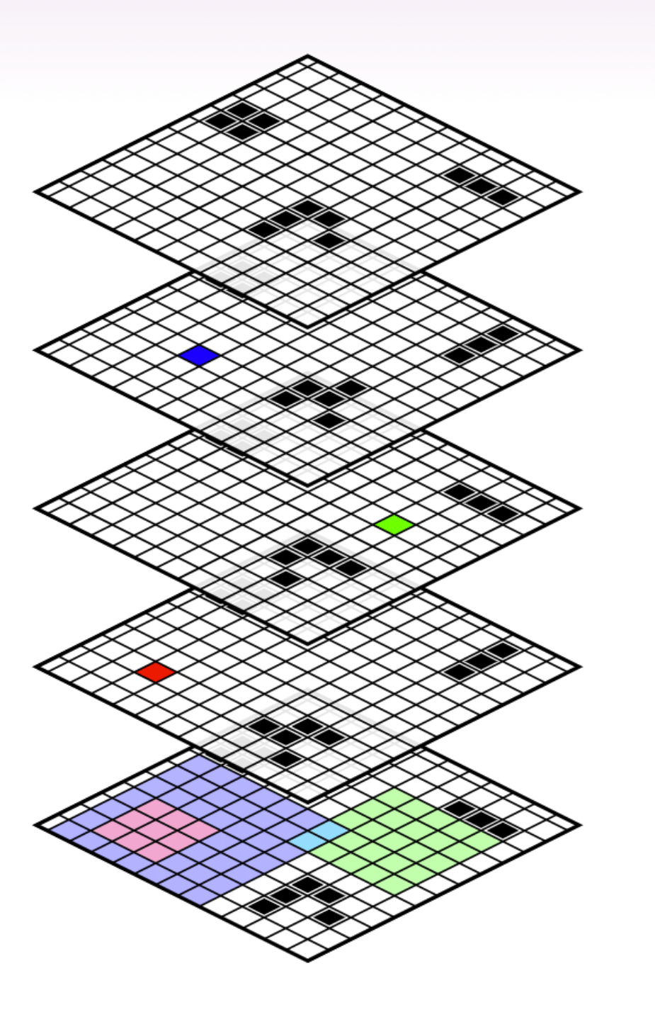
The lowest grid shows a section of the initial board state.
The blue, green, and red squares on the upper boards are (cell, time) pairs. Each square corresponds to a partition of the set of all Game of Life computations, “Is that cell alive or dead at the given time \(t\)?”
The history of that partition is going to be all the cells in the initial board that go into computing whether the cell is alive or dead at time \(t\) . It’s everything involved in figuring out that cell’s state. E.g., knowing the state of the nine light-red cells in the initial board always tells you the state of the red cell in the second board.
In this example, the partition corresponding to the red cell’s state is strictly before the partition corresponding to the blue cell. The question of whether the red cell is alive or dead is before the question of whether the blue cell is alive or dead.
Meanwhile, the question of whether the red cell is alive or dead is going to be orthogonal to the question of whether the green cell is alive or dead.
And the question of whether the blue cell is alive or dead is not going to be orthogonal to the question of whether the green cell is alive or dead, because they intersect on the cyan cells.
Generalizing the point, fix \(X=L_{(r_X,c_X,t_X)}, Y=L_{(r_Y,c_Y,t_Y)}\), where \((r_X,c_X,t_X),(r_Y,c_Y,t_Y)\in R\). Then:
- \(h^{F}(X)=\{L_{(r,c,0)}\in B\mid |r_X-r|\leq t_X,|c_X-c|\leq t_X\}\).
- \(X \ ᐸ^{F} \ Y\) if and only if \(t_X \ ᐸ \ t_Y\) and \(|r_Y-r_X|,|c_Y-c_X|\leq t_Y-t_X\).
- \(X \perp^F Y\) if and only if \(|r_Y-r_X|> t_Y+t_X\) or \(|c_Y-c_X|> t_Y+t_X\).
We can also see that the blue and green cells look almost orthogonal. If we condition on the values of the two cyan cells in the intersection of their histories, then the blue and green partitions become orthogonal. That’s what we’re going to discuss next.
| David Spivak: A priori, that would be a gigantic computation—to be able to tell me that you understand the factorization structure of that Game of Life. So what intuition are you using to be able to make that claim, that it has the kind of factorization structure you’re implying there?
Scott: So, I’ve defined the factorization structure. David Spivak: You gave us a certain factorization already. So somehow you have a very good intuition about history, I guess. Maybe that’s what I’m asking about. Scott: Yeah. So, if I didn’t give you the factorization, there’s this obnoxious number of factorizations that you could put on the set here. And then for the history, the intuition I’m using is: “What do I need to know in order to compute this value?” I actually went through and I made little gadgets in Game of Life to make sure I was right here, that every single cell actually could in some situations affect the cells in question. But yeah, the intuition that I’m working from is mostly about the information in the computation. It’s “Can I construct a situation where if only I knew this fact, I would be able to compute what this value is? And if I can’t, then it can take two different values.” David Spivak: Okay. I think deriving that intuition from the definition is something I’m missing, but I don’t know if we have time to go through that. Scott: Yeah, I think I’m not going to here. |
(Part 2, Main Body) · · · Conditional Orthogonality
 So, just to set your expectations: Every time I explain Pearlian causal inference to someone, they say that d-separation is the thing they can’t remember. d-separation is a much more complicated concept than “directed paths between nodes” and “nodes without any common ancestors” in Pearl; and similarly, conditional orthogonality will be much more complicated than time and orthogonality in our paradigm. Though I do think that conditional orthogonality has a much simpler and nicer definition than d-separation.
We’ll begin with the definition of conditional history. We again have a fixed finite set as our context. Let \(F=(S,B)\) be a finite factored set, let \(X,Y,Z\in\text{Part}(S)\), and let \(E\subseteq S\).
The conditional history of \(X\) given \(E\), written \(h^F(X|E)\), is the smallest set of factors \(H\subseteq B\) satisfying the following two conditions:
- For all \(s,t\in E\), if \(s\sim_{b} t\) for all \(b\in H\), then \(s\sim_X t\).
- For all \(s,t\in E\) and \(r\in S\), if \(r\sim_{b_0} s\) for all \(b_0\in H\) and \(r\sim_{b_1} t\) for all \(b_1\in B\setminus H\), then \(r\in E\).
The first condition is much like the condition we had in our definition of history, except we’re going to make the assumption that we’re in \(E\). So the first condition is: if all you know about an object is that it’s in \(E\), and you want to know which part it’s in within \(X\), it suffices for me to tell you which part it’s in within each factor in the history \(H\).
Our second condition is not actually going to mention \(X\). It’s going to be a relationship between \(E\) and \(H\). And it says that if you want to figure out whether an element of \(S\) is in \(E\), it’s sufficient to parallelize and ask two questions:
- “If I only look at the values of the factors in \(H\), is ‘this point is in \(E\)’ compatible with that information?”
- “If I only look at the values of the factors in \(B\setminus H\) , is ‘this point is in \(E\)’ compatible with that information?”
If both of these questions return “yes”, then the point has to be in \(E\).
I am not going to give an intuition about why this needs to be a part of the definition. I will say that without this second condition, conditional history would not even be well-defined, because it wouldn’t be closed under intersection. And so I wouldn’t be able to take the smallest set of factors in the subset ordering.
Instead of justifying this definition by explaining the intuitions behind it, I’m going to justify it by using it and appealing to its consequences.
We’re going to use conditional history to define conditional orthogonality, just like we used history to define orthogonality. We say that \(X\) and \(Y\) are orthogonal given \(E\subseteq S\), written \(X \perp^{F} Y \mid E\), if the history of \(X\) given \(E\) is disjoint from the history of \(Y\) given \(E\): \(h^F(X|E)\cap h^F(Y|E)=\{\}\).
We say \(X\) and \(Y\) are orthogonal given \(Z\in\text{Part}(S)\), written \(X \perp^{F} Y \mid Z\), if \(X \perp^{F} Y \mid z\) for all \(z\in Z\). So what it means to be orthogonal given a partition is just to be orthogonal given each individual way that the partition might be, each individual part in that partition.
I’ve been working with this for a while and it feels pretty natural to me, but I don’t have a good way to push the naturalness of this condition. So again, I instead want to appeal to the consequences.
(Part 2, Main Body) · · · Compositional Semigraphoid Axioms
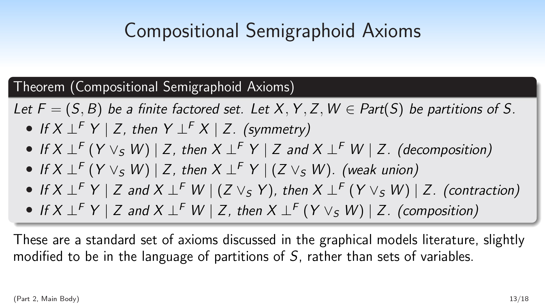 Conditional orthogonality satisfies the compositional semigraphoid axioms, which means finite factored sets are pretty well-behaved.
Let \(F=(S,B)\) be a finite factored set, and let \(X,Y,Z,W\in \text{Part}(S)\) be partitions of \(S\). Then:
- If \(X \perp^{F} Y \mid Z\), then \(Y \perp^{F} X \mid Z\). (symmetry)
- If \(X \perp^{F} (Y\vee_S W) \mid Z\), then \(X \perp^{F} Y \mid Z\) and \(X \perp^{F} W \mid Z\). (decomposition)
- If \(X \perp^{F} (Y\vee_S W) \mid Z\), then \(X \perp^{F} Y \mid (Z\vee_S W)\). (weak union)
- If \(X \perp^{F} Y \mid Z\) and \(X \perp^{F} W \mid (Z\vee_S Y)\), then \(X \perp^{F} (Y\vee_S W) \mid Z\). (contraction)
- If \(X \perp^{F} Y \mid Z\) and If \(X \perp^{F} W \mid Z\), then \(X \perp^{F} (Y\vee_S W) \mid Z\). (composition)
The first four properties here make up the semigraphoid axioms, slightly modified because I’m working with partitions rather than sets of variables, so union is replaced with common refinement. There’s another graphoid axiom which we’re not going to satisfy; but I argue that we don’t want to satisfy it, because it doesn’t play well with determinism.
The fifth property here, composition, is maybe one of the most unintuitive, because it’s not exactly satisfied by probabilistic independence.
Decomposition and composition act like converses of each other. Together, conditioning on \(Z\) throughout, they say that \(X\) is orthogonal to both \(Y\) and \(W\) if and only if \(X\) is orthogonal to the common refinement of \(Y\) and \(W\).
(Part 2, Main Body) · · · The Fundamental Theorem
 In addition to being well-behaved, I also want to show that conditional orthogonality is pretty powerful. The way I want to do this is by showing that conditional orthogonality exactly corresponds to conditional independence in all probability distributions you can put on your finite factored set. Thus, much like d-separation in the Pearlian picture, conditional orthogonality can be thought of as a combinatorial version of probabilistic independence.
A probability distribution on a finite factored set \(F=(S,B)\) is a probability distribution \(P\) on \(S\) that can be thought of as coming from a bunch of independent probability distributions on each of the factors in \(B\). So \(P(s)=\prod_{b\in B}P([s]_b)\) for all \(s\in S\).
This effectively means that your probability distribution factors the same way your set factors: the probability of any given element is the product of the probabilities of each of the individual parts that it’s in within each factor.
The fundamental theorem of finite factored sets says: Let \(F=(S,B)\) be a finite factored set, and let \(X,Y,Z\in \text{Part}(S)\) be partitions of \(S\). Then \(X \perp^{F} Y \mid Z\) if and only if for all probability distributions \(P\) on \(F\), and all \(x\in X\), \(y\in Y\), and \(z\in Z\), we have \(P(x\cap z)\cdot P(y\cap z)= P(x\cap y\cap z)\cdot P(z)\). I.e., \(X\) is orthogonal to \(Y\) given \(Z\) if and only conditional independence is satisfied across all probability distributions.
This theorem, for me, was a little nontrivial to prove. I had to go through defining certain polynomials associated with the subsets, and then dealing with unique factorization in the space of these polynomials; I think the proof was eight pages or something.
The fundamental theorem allows us to infer orthogonality data from probabilistic data. If I have some empirical distribution, or I have some Bayesian distribution, I can use that to infer some orthogonality data. (We could also imagine orthogonality data coming from other sources.) And then we can use this orthogonality data to get temporal data.
So next, we’re going to talk about how to get temporal data from orthogonality data.
(Part 2, Main Body) · · · Temporal Inference
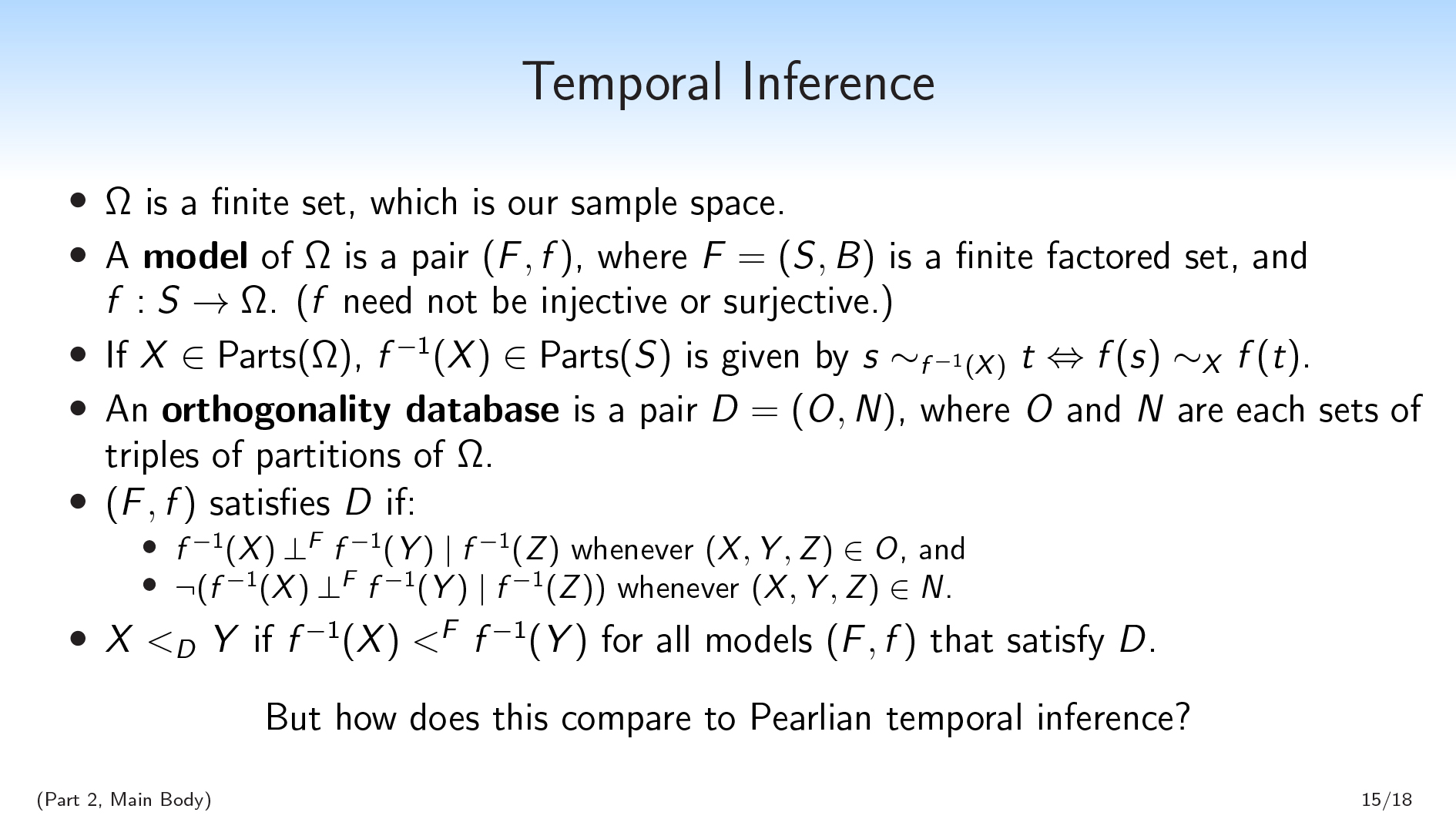 We’re going to start with a finite set \(\Omega\), which is our sample space.
One naive thing that you might think we would try to do is infer a factorization of \(\Omega\). We’re not going to do that because that’s going to be too restrictive. We want to allow for \(\Omega\) to maybe hide some information from us, for there to be some latent structure and such.
There may be some situations that are distinct without being distinct in \(\Omega\). So instead, we’re going to infer a factored set model of \(\Omega\): some other set \(S\), and a factorization of \(S\), and a function from \(S\) to \(\Omega\).
A model of \(\Omega\) is a pair \((F, f)\), where \(F=(S,B)\) is a finite factored set and \(f:S\rightarrow \Omega\). ( \(f\) need not be injective or surjective.)
Then if I have a partition of \(\Omega\), I can send this partition backwards across \(f\) and get a unique partition of \(S\). If \(X\in \text{Parts}(\Omega)\), then \(f^{-1}(X)\in \text{Parts}(S)\) is given by \(s\sim_{f^{-1}(X)}t\Leftrightarrow f(s)\sim_X f(t)\).
Then what we’re going to do is take a bunch of orthogonality facts about \(\Omega\), and we’re going to try to find a model which captures the orthogonality facts.
We will take as given an orthogonality database on \(\Omega\), which is a pair \(D = (O, N)\), where \(O\) (for “orthogonal”) and \(N\) (for “not orthogonal”) are each sets of triples \((X,Y,Z)\) of partitions of \(\Omega\). We’ll think of these as rules about orthogonality.
What it means for a model \((F,f)\) to satisfy a database \(D\) is:
- \(f^{-1}(X) \perp^{F} f^{-1}(Y) \mid f^{-1}(Z)\) whenever \((X,Y,Z)\in O\), and
- \(\) \(\lnot (f^{-1}(X) \perp^{F} f^{-1}(Y) \mid f^{-1}(Z))\) whenever \((X,Y,Z)\in N\).
So we have these orthogonality rules we want to satisfy, and we want to consider the space of all models that are consistent with these rules. And even though there will always be infinitely many models that are consistent with my database, if at least one is—you can always just add more information that you then delete with \(f\)—we would like to be able to sometimes infer that for all models that satisfy our database, \(f^{-1}(X)\) is before \(f^{-1}(Y)\).
And this is what we’re going to mean by inferring time. If all of our models \((F,f)\) that are consistent with the database \(D\) satisfy some claim about time \(f^{-1}(X) \ ᐸ^F \ f^{-1}(Y)\), we’ll say that \(X \ ᐸ_D \ Y\).
(Part 2, Examples) · · · Two Binary Variables (Pearl)
 So we’ve set up this nice combinatorial notion of temporal inference. The obvious next questions are:
- Can we actually infer interesting facts using this method, or is it vacuous?
- And: How does this framework compare to Pearlian temporal inference?
Pearlian temporal inference is really quite powerful; given enough data, it can infer temporal sequence in a wide variety of situations. How powerful is the finite factored sets approach by comparison?
To address that question, we’ll go to an example. Let \(X\) and \(Y\) be two binary variables. Pearl asks: “Are \(X\) and \(Y\) independent?” If yes, then there’s no path between the two. If no, then there may be a path from \(X\) to \(Y\), or from \(Y\) to \(X\), or from a third variable to both \(X\) and \(Y\).
In either case, we’re not going to infer any temporal relationships.
To me, it feels like this is where the adage “correlation does not imply causation” comes from. Pearl really needs more variables in order to be able to infer temporal relationships from more rich combinatorial structures.
However, I claim that this Pearlian ontology in which you’re handed this collection of variables has blinded us to the obvious next question, which is: is \(X\) independent of \(X \ \mathrm{XOR} \ Y\)?
In the Pearlian world, \(X\) and \(Y\) were our variables, and \(X \ \mathrm{XOR} \ Y\) is just some random operation on those variables. In our world, \(X \ \mathrm{XOR} \ Y\) instead is a variable on the same footing as \(X\) and \(Y\). The first thing I do with my variables \(X\) and \(Y\) is that I take the product \(X \times Y\) and then I forget the labels \(X\) and \(Y\).
So there’s this question, “Is \(X\) independent of \(X \ \mathrm{XOR} \ Y\)?”. And if \(X\) is independent of \(X \ \mathrm{XOR} \ Y\), we’re actually going to be able to conclude that \(X\) is before \(Y\)!
So not only is the finite factored set paradigm non-vacuous, and not only is it going to be able to keep up with Pearl and infer things Pearl can’t, but it’s going to be able to infer a temporal relationship from only two variables.
So let’s go through the proof of that.
(Part 2, Examples) · · · Two Binary Variables (Factored Sets)
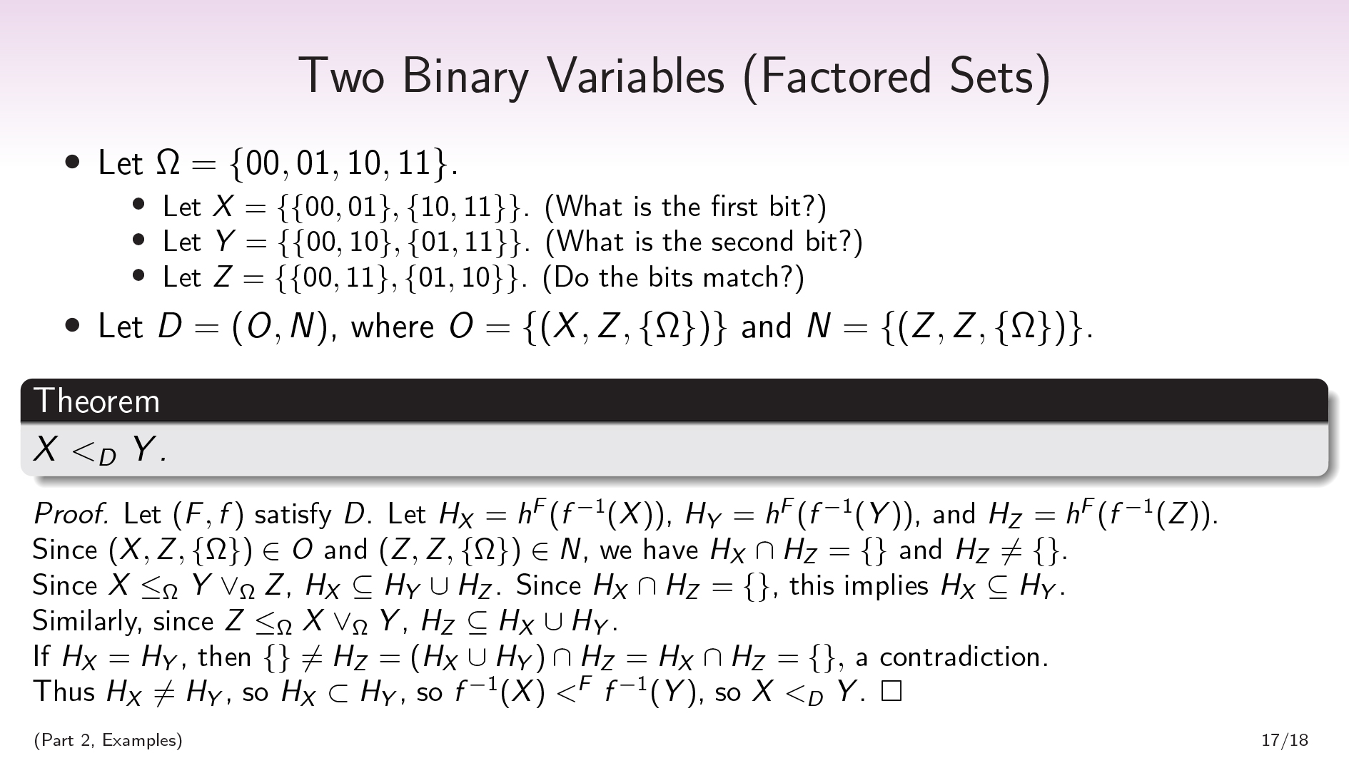
Let \(\Omega=\{00,01,10,11\}\), and let \(X\), \(Y\), and \(Z\) be the partitions (/questions):
- \(X = \{\{00,01\}, \{10,11\}\}\). (What is the first bit?)
- \(Y=\{\{00,10\}, \{01,11\}\}\). (What is the second bit?)
- \(Z=\{\{00,11\}, \{01,10\}\}\). (Do the bits match?)
Let \(D = (O,N)\), where \(O = \{(X, Z, \{\Omega\})\}\) and \(N = \{(Z, Z, \{\Omega\})\}\). If we’d gotten this orthogonality database from a probability distribution, then we would have more than just two rules, since we would observe more orthogonality and non-orthogonality than that. But temporal inference is monotonic with respect to adding more rules, so we can just work with the smallest set of rules we’ll need for the proof.
The first rule says that \(X\) is orthogonal to \(Z\). The second rule says that \(Z\) is not orthogonal to itself, which is basically just saying that \(Z\) is non-deterministic; it’s saying that both of the parts in \(Z\) are possible, that both are supported under the function \(f\). The \(\{\Omega\}\) indicates that we aren’t making any conditions.
From this, we’ll be able to prove that \(X \ ᐸ_D \ Y\).
Proof. First, we’ll show that that \(X\) is weakly before \(Y\). Let \((F,f)\) satisfy \(D\). Let \(H_X\) be shorthand for \(h^F(f^{-1}(X))\), and likewise let \(H_Y=h^F(f^{-1}(Y))\) and \(H_Z=h^F(f^{-1}(Z))\).
Since \((X,Z,\{\Omega\})\in O\), we have that \(H_X\cap H_Z=\{\}\); and since \((Z,Z,\{\Omega\})\in N\), we have that \(H_Z\neq \{\}\).
Since \(X\leq_{\Omega} Y\vee_{\Omega} Z\)—that is, since \(X\) can be computed from \(Y\) together with \(Z\)—\(H_X\subseteq H_Y\cup H_Z\). (Because a partition’s history is the smallest set of factors needed to compute that partition.)
And since \(H_X\cap H_Z=\{\}\), this implies \(H_X\subseteq H_Y\), so \(X\) is weakly before \(Y\).
To show the strict inequality, we’ll assume for the purpose of contradiction that \(H_X\) = \(H_Y\).
Notice that \(Z\) can be computed from \(X\) together with \(Y\)—that is, \(Z\leq_{\Omega} X\vee_{\Omega} Y\)—and therefore \(H_Z\subseteq H_X\cup H_Y\) (i.e., \(H_Z \subseteq H_X\) ). It follows that \(H_Z = (H_X\cup H_Y)\cap H_Z=H_X\cap H_Z\). But since \(H_Z\) is also disjoint from \(H_X\), this means that \(H_Z = \{\}\), a contradiction.
Thus \(H_X\neq H_Y\), so \(H_X \subset H_Y\), so \(f^{-1}(X) \ ᐸ^F \ f^{-1}(Y)\), so \(X \ ᐸ_D \ Y\). □
When I’m doing temporal inference using finite factored sets, I largely have proofs that look like this. We collect some facts about emptiness or non-emptiness of various Boolean combinations of histories of variables, and we use these to conclude more facts about histories of variables being subsets of each other.
I have a more complicated example that uses conditional orthogonality, not just orthogonality; I’m not going to go over it here.
One interesting point I want to make here is that we’re doing temporal inference—we’re inferring that \(X\) is before \(Y\)—but I claim that we’re also doing conceptual inference.
Imagine that I had a bit, and it’s either a 0 or a 1, and it’s either blue or green. And these two facts are primitive and independently generated. And I also have this other concept that’s like, “Is it grue or bleen?”, which is the \(\mathrm{XOR}\) of blue/green and 0/1.
There’s a sense in which we’re inferring \(X\) is before \(Y\) , and in that case, we can infer that blueness is before grueness. And that’s pointing at the fact that blueness is more primitive, and grueness is a derived property.
In our proof, \(X\) and \(Z\) can be thought of as these primitive properties, and \(Y\) is a derived property that we’re getting from them. So we’re not just inferring time; we’re inferring facts about what are good, natural concepts. And I think that there’s some hope that this ontology can do for the statement “you can’t really distinguish between blue and grue” what Pearl can do to the statement “correlation does not imply causation”.
(Part 2, Main Body) · · · Applications / Future Work / Speculation
 The future work I’m most excited by with finite factored sets falls into three rough categories: inference (which involves more computational questions), infinity (more mathematical), and embedded agency (more philosophical).
Research topics related to inference:
- Decidability of Temporal Inference
- Efficient Temporal Inference
- Conceptual Inference
- Temporal Inference from Raw Data and Fewer Ontological Assumptions
- Temporal Inference with Deterministic Relationships
- Time without Orthogonality
- Conditioned Factored Sets
There are a lot of research directions suggested by questions like “How do we do efficient inference in this paradigm?”. Some of the questions here come from the fact that we’re making fewer assumptions than Pearl, and are in some sense more coming from the raw data.
Then I have the applications that are about extending factored sets to the infinite case:
- Extending Definitions to the Infinite Case
- The Fundamental Theorem of Finite-Dimensional Factored Sets
- Continuous Time
- New Lens on Physics
Everything I’ve presented in this talk was under the assumption of finiteness. In some cases this wasn’t necessary—but in a lot of cases it actually was, and I didn’t draw attention to this.
I suspect that the fundamental theorem can be extended to finite-dimensional factored sets (i.e., factored sets where \(|B|\) is finite), but it can not be extended to arbitrary-dimension factored sets.
And then, what I’m really excited about is applications to embedded agency:
- Embedded Observations
- Counterfactability
- Cartesian Frames Successor
- Unraveling Causal Loops
- Conditional Time
- Logical Causality from Logical Induction
- Orthogonality as Simplifying Assumptions for Decisions
- Conditional Orthogonality as Abstraction Desideratum
I focused on the temporal inference aspect of finite factored sets in this talk, because it’s concrete and tangible to be able to say, “Ah, we can do Pearlian temporal inference, only we can sometimes infer more structure and we rely on fewer assumptions.”
But really, a lot of the applications I’m excited about involve using factored sets to model situations, rather than inferring factored sets from data.
Anywhere that we currently model a situation using graphs with directed edges that represent information flow or causality, we might instead be able to use factored sets to model the situation; and this might allow our models to play more nicely with abstraction.
I want to build up the factored set ontology as an alternative to graphs when modeling agents interacting with things, or when modeling information flow. And I’m really excited about that direction.